[언어지능 딥러닝] 38일차 - 딥러닝의 역사~GAN 까지 + 코드

티스토리 뷰

프로젝트/에이블스쿨

[언어지능 딥러닝] 38일차 - 딥러닝의 역사~GAN 까지 + 코드

sikaro 2024. 4. 16. 17:23

복습

TF-IDF로 벡터화한 값은 자카드 유사도를 제외한 모든 유사도 판단에서 사용한다.

코사인 유사도 - 직관적인 유사도 값을 가진다.

회사에서 코딩하는 거랑 연구하는 것이랑 다르다.

소프트웨어 값을 계속 바꿔도 소리가 안잡힌다.

pcb 하드 웨어에서 전력이 문제

업체 부르면 해결

회사는 공부를 가르쳐 주는 게 아니라, 데드라인을 맞추는 게 중요하다.

남의 코드를 잽싸게 보고, 거기에 내가 원하는 코드를 빠르게 넣는게 중요하다.

남의 코드를 많이 돌려보면서 눈에 익어서, github 같은 코드 중에서 빠르게 고칠 수 있는 능력이 제일 좋다.

소프트웨어공학 - 에자일 방법론, 디자인 패턴

회사에서는 제일 중요한 게 이것이다.

Word Embedding

신경망을 만들어서 학습을 시켰다.

일단 원핫 인코딩을 만들어서 다른 사람이 임베딩한 결과(히든 레이어)를 가져다가 쓴다.

단어에 따라서 해당 윈도우 범위에 따라 그를 경계로 하여 해당 단어에 대한 관계 output이 달라진다.

KoNLPy(Hannanum)

.tag에 Okt가 있고, Hannanum이 있다.

Hannanum.analyze("") = 전체분석

morphs=다 쪼개서 리스트로 만든다.

nouns = 명사만 추출

pos 명사인지, 뭔지 형태소를 넣어준다.

KoNLpy(Kkma)

pprint가 있다.

pprint는 하나의 튜플마다 줄을 바꿔준다.

kkma.morphs, noun,pos 등

KoNLPy(Komoran)

여기도 morphs,nouns,pos

그런데 userdic='lib/dic.txt') # lib라는 폴더 안에 idc.txt를 만든다. 그 안에

단어1 NNP

단어2 NNP

단어 3 NNG

단어 4 NNP

라이브러리가 미처 영화제목을 다 모르더라도 등록된 대로 인식을 한다.

미리 언어 사전을 만들어놓고 시작을 한다.

News parsing

첫번째 방법

from urllib.request import urlopen
from bs4 import BeautifulSoup

#file을 open하고, 해당 url에 대해서 urlopen해서 그 링크를 넣으면 텍스트가 나온다.
url = urlopen('https://www.etnews.com/20240416000215?mc=em_004_00001')
soup =BeautifulSoup(url, "lxml")

title = soup.find_all("div", {"class":"article_title"})
contents = soup.find_all("div",{"class":"article_txt"})

print(title)
print(contents)

find 뒤에 .get_text(strip=True)를 붙여주시면 텍스트만 나옵니다!
혹은 preprocessing 하면 된다.

title = soup.find('div', {'class':'article_title'}).get_text(strip=True) 
contents = soup.find('div', {'class':'article_txt'}).get_text(strip=True)

a = Article(url2,...)

b= Article(url3,...)

a.parse

b.parse

내일은 IMDB 감상평에 대한 실습

감정이 다 드러나지 않는다.

그러나 영화는 감정이 드러난다.

말 그대로 감정 분류기

스탠포드에서 다운로드하여 압축을 푸는 것으로부터 시작한다.

긍정은 1 부정은 0

import os # 경로를 지정하거나 연산에 쓰기 위하여
import re # regular expression 주어진 규칙에 맞는 언어 연산
import pandas as pd # 데이터처리 및 데이터과학을 위한 라이브러리
import tensorflow as tf # 데이터 다운받는 용도로 필요
from tensorflow.keras import utils # 데이터 다운받는 용도로 필요

# IMBD 데이터 다운로드
data_set = tf.keras.utils.get_file(
    fname = "imdb.tar.gz", # 다운받은 파일의 이름
    origin = "http://ai.stanford.edu/~amaas/data/sentiment/aclImdb_v1.tar.gz",
    extract = True)
def directory_data(directory):
  data = {}
  data["review"] = []
  for file_path in os.listdir(directory):
    with open(os.path.join(directory, file_path), "r", encoding='utf-8') as file:
      data["review"].append(file.read())
  return pd.DataFrame.from_dict(data)
def data(directory):
  pos_df = directory_data(os.path.join(directory, "pos"))
  neg_df = directory_data(os.path.join(directory, "neg"))
  pos_df["sentiment"] = 1
  neg_df["sentiment"] = 0
  return pd.concat([pos_df, neg_df])
train_df = data(os.path.join(os.path.dirname(data_set), "aclImdb", "train"))
test_df = data(os.path.join(os.path.dirname(data_set), "aclImdb", "test"))
imdb_pd = pd.concat([train_df, test_df])
imdb_pd.head()

불용어는 불용어 사전을 가져와야 한다.

from nltk.corpus import stopwords #불용어 사전을 가젼돠
import nltk
nltk.download('stopwords') #불용어를 다운 받음
set_stopwords= set(stopwords.words('english')) #영어로 된 불용어를 가져다 집합으로 구성

def preprocessing(review,remove_stopwords=True):
    review_text = BeautifulSoup(review,'html5lib').get_text() #html 태그 제거
    review_text = re.sub("[^a-zA~Z]", " ", review_text) #[]는 제외하고라는 뜻, a-z, A~Z 빼고는 빈칸으로 대체한다. review_text안의 글자를 대체
    if remove_stopwords: #만약에 이 함수를 쓸 데에 stopwords를 제거하려고 한다면
        words = review_text.split() #현재 HTML 제거하고, 알파벳들로만 구성된 리뷰글을 쪼개서 리스트로 만든다.
        #위의 split의 예시는 [I,am,a,boy]
        #set_stopwords에 속하지 않으면 불용어가 아니다.
        words =[w for w in words if not w in set_stopwords]
        revied_text = ' '.join(words)
        #결과적으로 'I boy'가 된다 
    review_text = review_text.lower()
    return review_text
list_reviews = list(imdb_pd['review'])
print(list_reviews[0])
print(preprocessing(list_reviews[0]))

LinearRegression - tensorflow

Cost(W,b) Cost함수)

grdient decent

cose 함수의 기울기가 0이 되는 지점을 찾는다.

기울기가 크면 클수록 많이 보정(learning rate)해서 빼주고,

작으면 작을수록 적게 보정해서 빼준다.

W <= W- alpha(a/aw * cost(W))

alpha 값을 잘 조절해서 쓴다.

adam은 2차원 미분이라 이미지에 특화되어 있다.

import tensorflow as tf
import numpy as np

# 데이터 정의
x_data = np.array([[1,1],[2,2],[3,3]], dtype=np.float32)
y_data = np.array([[10],[20],[30]], dtype=np.float32)

# 선형 회귀 모델 정의
def model_LinearRegression(x):
    return tf.matmul(x, w) + b

# 비용 함수 정의
def cost_LinearRegression(model_x):
    return tf.reduce_mean(tf.square(model_x - y_data))

# 모델 최적화 함수 정의
def train_optimization(x):
    with tf.GradientTape() as g:
        model = model_LinearRegression(x)
        cost = cost_LinearRegression(model)
        gradients = g.gradient(cost, [w,b])
    tf.optimizers.SGD(0.01).apply_gradients(zip(gradients, [w,b]))

# 모델 초기화
w = tf.Variable(tf.random.normal([2,1]))
b = tf.Variable(tf.random.normal([1]))

# 최적화 반복
for step in range(2001):
    train_optimization(x_data)

# 테스트 데이터에 모델 적용
x_test = np.array([[4],[4]], dtype=np.float32)
model_test = model_LinearRegression(x_test)

# 결과 출력
print("model for [4,4]: ", model_test.numpy())

matmul은 행렬 곱셈을 수행하는 함수다.

matmul(x, w) 함수는 입력 데이터 행렬 x와 가중치 행렬 w를 곱하여 결과 행렬을 반환

한마디로, 코드는 텐서에 대한 식을 그대로 표현하는 것 뿐이다.

pytorch

import torch

# 데이터 정의
x_train = torch.FloatTensor([[1,1],[2,2],[3,3]])
y_train = torch.FloatTensor([[10],[20],[30]])

# 가중치 및 편향 초기화
W = torch.randn([2,1], requires_grad=True)
b = torch.randn([1], requires_grad=True)

# 옵티마이저 설정
optimizer = torch.optim.SGD([W, b], lr=0.01)

# 선형 회귀 모델 정의
def model_LinearRegression(x):
    return torch.matmul(x, W) + b

# 학습
for step in range(2000):
    prediction = model_LinearRegression(x_train)
    cost = torch.mean((prediction - y_train) ** 2) #predction 해서 나온 값을, cost 함수로 만든다.
    optimizer.zero_grad() #그라디언트 초기화
    cost.backward() #역전파 업데이트
    optimizer.step() #옵티마이저 사용

# 테스트 데이터에 모델 적용
x_test = torch.FloatTensor([[4,1]]) #테스트 값을 텐서로 만든다.
model_test = model_LinearRegression(x_test) #해당 값을 모델에 적용

# 결과 출력
print("Model with [4,1] (expectation: 40): ", model_test.detach().item())

각각의 결과는 이렇다.

x_train=
tensor([[1., 1.],
        [2., 2.],
        [3., 3.]])
        
y_train=
tensor([[10.],
        [20.],
        [30.]])
        
W , b

(tensor([[-2.4213],
         [-0.0446]], requires_grad=True),
 tensor([0.0149], requires_grad=True))
 

optimizer = torch.optim.SGD([W, b], lr=0.01)
 SGD (
Parameter Group 0
    dampening: 0
    differentiable: False
    foreach: None
    lr: 0.01
    maximize: False
    momentum: 0
    nesterov: False
    weight_decay: 0
)

keras

import numpy as np
import matplotlib.pyplot as plt
from keras.models import Sequential
from keras.layers import Dense

# 데이터 정의
x_data = np.array([[1], [2], [3]])
y_data = np.array([[10], [20], [30]])

# 모델 구성
model = Sequential()
model.add(Dense(1, input_dim=1))

# 모델 컴파일
model.compile(loss='mse', optimizer='adam')

# 모델 학습
model.fit(x_data, y_data, epochs=1000, verbose=0)

# 모델 요약
model.summary()

# 추론
print(model.get_weights())
print(model.predict(np.array([[4]])))

# 시각화
plt.scatter(x_data, y_data)
plt.plot(x_data, model.predict(x_data), 'r')
plt.grid(True)
plt.show()

이진 분류 모델

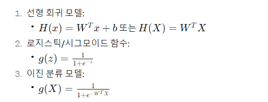
예시는 선형 회귀 모델을 넣었다고 했을 때 나오는 이진 분류 모델의 함수이다.

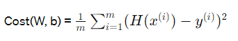
Cost(W,b)는 한마디로 mse

선형 모델에서는 Gradient Descent Method가 사용될 수 있다. 왜냐면 Cost(W,b)가 convex(local minimum이 global minumum)하기 때문이다. convex는 볼록한 함수라는 뜻이다. 임의의 두 점을 선택했을 때 그 두점을 연결하는 선 위의 모든 점들이 해당 함수의 값보다 작거나 같다.

하지만 이진 분류 모델은 Cost(W,b)에 넣었을 때 non-convex) 하다. 그렇기에 새로운 Cost Function이 필요하다.

W 값에 따른 J(W) 함수(오차함수) - 그래프를 그렸을 때, 전체 그래프에서 해당 오차 값이 실제로 가장 적은 곳이 Gloabal cost minimum이다.

지역적으로 오차가 갇히는 곳이 생기는데, 그곳이 local cost minimum이다.

그러나 어찌되었던 Gradient Decent를 쓰려면 convex가 되어야, J(W)함수가 생성되어 사용할 수 있다.

그렇기에 mse라는 cost function을 변환한다.

이진 분류에 사용되는 비용 함수가 c(H(x),y)가 된다.

-log를 쓰는 이유는 0에 가까워질수록 무한이어야 하고, x가 높아질수록 0이 되어야 하기 때문이다.

그렇게 두 개를 합쳐서, cost function을 결정하게 된다.

가중치 업데이트를 다음과 같이 진행하게 된다.

한마디로 W를 편미분하여 alpha의 learning rate를 반영한다.

이진 분류의 코드 -tensorflow

import tensorflow as tf
import numpy as np

# 데이터 정의
x_train = np.array([[1,2],[2,3],[3,4],[4,5],[6,2]], dtype=np.float32)
y_train = np.array([[0],[0],[0],[1],[1]], dtype=np.float32)

# 가중치 및 편향 초기화
w = tf.Variable(tf.random.normal([2,1]))
b = tf.Variable(tf.random.normal([1]))

# 이진 분류 모델 정의
def model_BinaryClassification(x):
    return tf.sigmoid(tf.matmul(x, w) + b)

# 이진 분류 모델 비용 함수 정의
def cost_BinaryClassification(model_x):
    return tf.reduce_mean(-1 * y_train * tf.math.log(model_x) - (1 - y_train) * tf.math.log(1 - model_x))

# 모델 최적화 함수 정의
def train_optimization(x):
    with tf.GradientTape() as g:
        model = model_BinaryClassification(x)
        cost = cost_BinaryClassification(model)
        gradients = g.gradient(cost, [w,b])
    tf.optimizers.SGD(0.01).apply_gradients(zip(gradients, [w,b]))


# 학습
for step in range(200):
    train_optimization(x_train)
    # 중간 결과 출력
    if (step+1) % 100 == 0:
        prediction = model_BinaryClassification(x_train)
        accuracy = tf.reduce_mean(tf.cast(tf.equal(tf.round(prediction), y_train), dtype=tf.float32))
        loss = cost_BinaryClassification(prediction)
        print("step: {}, accuracy: {}, loss: {}".format(step+1, accuracy.numpy().flatten()[0], loss))

# 테스트 데이터에 모델 적용
x_test = np.array([[5,1]], dtype=np.float32)
model_test = model_BinaryClassification(x_test)
print("model for [5,1]: ", model_test.numpy())

선형 회귀 모델을 sigmoid에 넣는다.

reduce_mean을 통해, 해당 모델에서 나온 prediction과 y_train을 통해 손실함수를 구한다.

reduce_mean은 주어진 텐서의 모든 요소에 대한 평균 값을 계산하여 반환.

그렇게 구한 함수를 업데이트 해가면서 구한다.

pytorch

import torch
import numpy as np

# 데이터 정의
x_train = torch.FloatTensor([[1,2],[2,3],[3,4],[4,4],[5,3],[6,2]])
y_train = torch.FloatTensor([[0],[0],[0],[1],[1],[1]])

# 가중치 및 편향 초기화
w = torch.randn([2,1], requires_grad=True)
b = torch.randn([1], requires_grad=True)
optimizer = torch.optim.SGD([w, b], lr=0.01)

# 이진 분류 모델 정의
def model_BinaryClassification(x):
    return torch.sigmoid(torch.matmul(x, w) + b)

# 학습
for step in range(2000):
    prediction = model_BinaryClassification(x_train)
    cost = torch.mean((-1) * y_train * torch.log(prediction) + (-1) * (1 - y_train) * torch.log(1 - prediction))
    optimizer.zero_grad()
    cost.backward()
    optimizer.step()

# 테스트 데이터에 모델 적용
x_test = torch.FloatTensor([[6,1]])
model_test = model_BinaryClassification(x_test)
print("Model with [6,1] (expectation: 1): ", torch.round(model_test).detach().item())

tensorflow와 똑같이 정의할 수 있다.

혹은, 다음과 같이 class를 이용할 수도 있다.

import torch
import torch.nn as nn
import torch.nn.functional as F
import numpy as np

# 데이터 정의
x_train = torch.FloatTensor([[1,2],[2,3],[3,4],[4,4],[5,3],[6,2]])
y_train = torch.FloatTensor([[0],[0],[0],[1],[1],[1]])

# 이진 분류 모델 클래스 정의
class BinaryClassification(nn.Module):
    def __init__(self):
        super().__init__()
        self.linear1 = nn.Linear(2, 3)
        self.linear2 = nn.Linear(3, 1)
        self.sigmoid = nn.Sigmoid()

    def forward(self, x):
        x = self.sigmoid(self.linear2(self.sigmoid(self.linear1(x))))
        return x

# 모델 및 최적화 함수 초기화
model_BinaryClassification = BinaryClassification()
optimizer = torch.optim.SGD(model_BinaryClassification.parameters(), lr=0.01)

# 학습
for step in range(2000):
    prediction = model_BinaryClassification(x_train)
    cost = F.binary_cross_entropy(prediction, y_train)
    optimizer.zero_grad()
    cost.backward()
    optimizer.step()

# 테스트 데이터에 모델 적용
x_test = torch.FloatTensor([[6,1]])
model_test = model_BinaryClassification(x_test)
print("Model with [6,1] (expectation: 1): ", torch.round(model_test).detach().item())

keras

keras로 하면 훨씬 쉬워진다.

import numpy as np
from keras.models import Sequential
from keras.layers import Dense

# 데이터 정의
x_data = np.array([[1,2],[2,3],[3,4],[4,3],[5,3],[6,2]])
y_data = np.array([[0], [0], [0], [1], [1], [1]])

# 모델 구성
model = Sequential()
model.add(Dense(1, activation='sigmoid', input_dim=2))

# 모델 컴파일 및 학습
model.compile(loss='binary_crossentropy', optimizer='sgd', metrics=['accuracy'])
model.fit(x_data, y_data, epochs=10000, verbose=1)

# 모델 요약 출력
model.summary()

# 추론
print(model.get_weights())
print(model.predict(x_data))

Softmax Classification 이론

다중 분류에서 각각에 대한 sigmoid를 하게 되면, 비율이 맞지 않는 문제가 생긴다.

그렇기에 확률적인 계산을 통해 전체가 1이 되도록 만든다.

tensorflow로는 tf.nn의 softmax_cross_entropy를 쓴다.

import tensorflow as tf
import numpy as np

x_train = np.array([[1,1,1,1,1],[2,2,2,2,2],[3,3,3,3,3],[4,4,4,4,4],[5,5,5,5,5],[1,2,3,4,5],[5,4,3,2,1],[1,0,0,0,1],[0,0,0,0,0]], dtype=np.float32)
y_train = np.array([[1,0,0],[1,0,0],[1,0,0],[1,0,0],[1,0,0],[0,1,0],[0,1,0],[0,0,1],[0,0,1]], dtype=np.float32)

x_test = np.array([[1,8,8,8,1]], dtype=np.float32)
y_test = np.array([[1,0,0]], dtype=np.float32)

w = tf.Variable(tf.random.normal([5,3]))
b = tf.Variable(tf.random.normal([3]))

def model_SoftmaxClassificationLC(x):
    return tf.matmul(x,w)+b

def cost_SoftmaxClassification(model_x):
    return tf.reduce_mean(tf.nn.softmax_cross_entropy_with_logits(logits=model_x, labels=y_train))

def train_optimization(x):
    with tf.GradientTape() as g:
        model_lc = model_SoftmaxClassificationLC(x)
        cost = cost_SoftmaxClassification(model_lc)
    gradients = g.gradient(cost, [w,b])
    tf.optimizers.SGD(0.01).apply_gradients(zip(gradients, [w,b]))

for step in range(2001):
    train_optimization(x_train)
    if step % 100 == 0:
        pred = model_SoftmaxClassificationLC(x_train)
        pred = tf.nn.softmax(pred)
        correct = tf.equal(tf.argmax(pred, 1), tf.argmax(y_train, 1))
        accuracy = tf.reduce_mean(tf.cast(correct, tf.float32))
        loss = cost_SoftmaxClassification(model_SoftmaxClassificationLC(x_train))
        print("Step: {},\t Accuracy: {},\t Loss: {}".format(step,accuracy.numpy().flatten(),loss))

print("model for input : ", tf.argmax(model_SoftmaxClassificationLC(x_test), 1).numpy())
print("label for input : ", tf.argmax(y_test, 1).numpy())

pytorch

import torch
import torch.nn as nn
import torch.nn.functional as F
import numpy as np

x_train = torch.FloatTensor([[1,1,1,1,1],[2,2,1,2,2],[3,3,1,3,3],[4,4,1,4,4],[5,5,1,5,5],[1,2,3,4,5],[5,4,3,2,1],[1,0,0,0,1],[0,0,0,0,0]])
y_train = torch.FloatTensor([[1,0,0],[1,0,0],[1,0,0],[1,0,0],[1,0,0],[0,1,0],[0,1,0],[0,0,1],[0,0,1]])

W = torch.randn([5,3], requires_grad=True)
b = torch.randn([3], requires_grad=True)
optimizer = torch.optim.SGD([W, b], lr=0.01)

def model_SoftmaxClassification(x):
    return F.softmax(torch.matmul(x, W) + b)

for step in range(50000):
    prediction = model_SoftmaxClassification(x_train)
    cost = F.cross_entropy(prediction, torch.argmax(y_train, 1))
    optimizer.zero_grad()
    cost.backward()
    optimizer.step()

x_test = torch.FloatTensor([[1,8,8,8,1]])
model_test = model_SoftmaxClassification(x_test)
index = torch.argmax(model_test.detach(), 1).item()

if index == 0:
    print("Model with [1,8,8,8,1] is A.")
elif index == 1:
    print("Model with [1,8,8,8,1] is B.")
elif index == 2:
    print("Model with [1,8,8,8,1] is C.")

nn.module 객체를 상속받아서, class로도 만들 수 있다.

import torch
import torch.nn as nn
import torch.nn.functional as F
import numpy as np

x_train = torch.FloatTensor([[1,1,1,1,1],[2,2,1,2,2],[3,3,1,3,3],[4,4,1,4,4],[5,5,1,5,5],[1,2,3,4,5],[5,4,3,2,1],[1,0,0,0,1],[0,0,0,0,0]])
y_train = torch.FloatTensor([[1,0,0],[1,0,0],[1,0,0],[1,0,0],[1,0,0],[0,1,0],[0,1,0],[0,0,1],[0,0,1]])

class class_SoftmaxClassification(nn.Module):
    def __init__(self):
        super().__init__()
        self.linear = nn.Linear(5, 3)
    
    def forward(self, x):
        return F.softmax(self.linear(x))

model_SoftmaxClassification = class_SoftmaxClassification()
optimizer = torch.optim.SGD(model_SoftmaxClassification.parameters(), lr=0.01)

for step in range(50000):
    prediction = model_SoftmaxClassification(x_train)
    cost = F.cross_entropy(prediction, torch.argmax(y_train, 1))
    optimizer.zero_grad()
    cost.backward()
    optimizer.step()

x_test = torch.FloatTensor([[1,8,8,8,1]])
model_test = model_SoftmaxClassification(x_test)
index = torch.argmax(model_test.detach(), 1).item()

if index == 0:
    print("Model with [1,8,8,8,1] is A.")
elif index == 1:
    print("Model with [1,8,8,8,1] is B.")
elif index == 2:
    print("Model with [1,8,8,8,1] is C.")

keras의 경우, 마지막 레이어의 activation만 softmax로 바꾸면 된다.

ANN(인공신경망) 이론

Application to Ligic Gate Design

AND gate =

인공신경망 레이어 1개 당, 선을 하나씩 긋는다.

하나씩 그으면서 해당 차원을 이동시켜서 XOR 문제를 해결할 수 있는 방법으로 만들어진다.

실제로 ANN을 solving 하는 방법

(x1,x2) =(0,0)

(0,0) * (5,5) + -8 = -8, y1=sigmoid(-8) ~=0(시그모이드에 -값이 들어왔으므로, 무조건 0.5보다 작다)

(0,0) * (-7,-7) + 3 = 3, y2=sigmoid(3) ~=1

(y1,y2) * (-11,-11) +6 = -11 +6 = -5 , y=sigmoid(-5)~=0

XOR = 0,0이 들어왔을 때 0이 나온다

0,1이 들어왔을 때 1이 나온다.

1,0이 들어왔을 때 1이 나온다

1,1이 들어왔을 때 0이 나온다.

즉, 두개가 같으면 0이 나온다.

이러한 문제를 풀기 위한 은닉층 구조가 ANN이다.

처음에 시그모이드를 통과했을 때 0이 나온다.

두번쨰 시그모이드를 통과했을 때 1이 나온다.

그러면 y1,y2가 0,1이 되고, 해당 벡터를 가중치를 곱해주면 최종값이 나오고, 그 최종값을 시그모이드 함수에 출력시켜 XOR 문제(분류 문제)를 푼다

3 , 4,4,1의 input,은닉층 2개, output layer가 있을 때,

경사하강법으로 한 번의 점프를 뛸 때에 몇 개의 신경망 내의 파라미터가 업데이트 되는가?

입력층과 첫 번째 은닉층 사이의 가중치 행렬: 3 x 4 = 12개의 가중치 파라미터
첫 번째 은닉층의 bias 벡터: 4개의 bias 파라미터
첫 번째 은닉층과 두 번째 은닉층 사이의 가중치 행렬: 4 x 4 = 16개의 가중치 파라미터
두 번째 은닉층의 bias 벡터: 4개의 bias 파라미터
두 번째 은닉층과 출력층 사이의 가중치 행렬: 4 x 1 = 4개의 가중치 파라미터
출력층의 bias 스칼라: 1개의 bias 파라미터
따라서, 경사하강법으로 한 번의 점프를 할 때 총 41개의 신경망 내 파라미터가 업데이트됩니다.

import torch

# 학습 데이터 설정
x_train = torch.FloatTensor([[0,0], [0,1], [1,0], [1,1]]) # XOR 문제의 입력
y_train = torch.FloatTensor([[0], [1], [1], [0]]) # XOR 문제의 정답

# 모델 초기화
W_h = torch.randn([2,3], requires_grad=True)
b_h = torch.randn([3], requires_grad=True)
W_o = torch.randn([3,1], requires_grad=True)
b_o = torch.randn([1], requires_grad=True)

# 옵티마이저 설정
optimizer = torch.optim.SGD([W_h, W_o, b_h, b_o], lr=0.01)

# 시그모이드 함수 정의
#def sigmoid(x):
#   return 1 / (1 + torch.exp(-x))

# 인공 신경망 정의
def H(x):
    HL1 = torch.sigmoid(torch.matmul(x, W_h) + b_h)
    return torch.sigmoid(torch.matmul(HL1, W_o) + b_o)

# 모델 학습
for step in range(50000):
    optimizer.zero_grad()
    cost = -torch.mean(y_train * torch.log(H(x_train)) + (1 - y_train) * torch.log(1 - H(x_train)))
    cost.backward()
    optimizer.step()

# 학습 결과 출력
print(H(x_train))

하나의 은닉층 뉴런당 어떤 연산을 거치든 나오는 연산의 값은 1개이다.

즉, 아무리 뉴런을 모아도 1차원으로 만들어진다. (n*1)

인공신경망의 단점 = 레이어를 많이 쌓지 못한다. > ReLU 함수로 극복

또한, 2차원 이상 처리 불가하다. => CNN으로 극복

현업에서는 실제 데이터를 어떻게 할 수 있는 방법이 없다.

데이터 100개 짜리가 들어오면 최소한 100의 뉴런 개수를 맞춰줘라. 데이터가 압축된다.-> 정보의 소실

RNN

시퀀스 데이터에 제일 좋다.

전의 단어에 대한 고려를 해서, 다음 단어가 나온다.

그렇기에 전의 값에 대한 고려를 후의 단어로 이어지게 해야 한다. ANN,CNN은 이게 불가능하다.

혼자 Input이 아니라, 전 시간의 신경망도 Input이 들어와야 한다.

즉, x0->은닉층1 ->y0가 나왔다면,

은닉층 1과 x1이 은닉층 2로 들어가서 y1이 나온다.

그렇게 영향력 있도록 행사한다. 즉, input이 2개가 들어가는 함수인 것이다.

그런데 이 input이 실현되려면, 결국 W의 가중치 벡터를 곱해줘야 하고, 해당 코스트 함수에 대한 벡터를 만들어야 한다.

따라서 다음과 같이 비용함수를 만든다.

ht-1이 5차원이고, xt가 10차원이라고 하자.

그러면 차원을 맞춰줘야 한다.

그렇기에 Whh,Wxh를 쓰고 activation인 tanh로 감싸주면, 그라디언트를 실행할 수 있다. (a * (Wx+b) 라고 생각하면 쉽다)

그렇게 Why라는 새로운 가중치 행렬을 곱해주면 yt가 된다. 이때 ht는 5차원이다.

이때 xt를 10차원으로 넣어주었으므로, 다시 복원하려면 10차원으로 만들어주기 위해 Why를 곱해주는 것이다.

여기서 출력 결과는 2개이다.

다음에 전달될 ht, 그리고 yt

yt, ht가 의미는 같은건데 표현식을 다르게 해주는 거여서 행렬 하나 추가하는 것이다.

keras의 simplernn에서는 return_sequence=True는 저장해둔 전체 벡터를 반환한다.(y0,y1...yt)

False로 하면 마지막 yt만 나온다.

따라서 fully connected layer는 결국 Why를 전부 묶어준 것이다.

RNN의 사용쳐

Image Captioning - one to many

Deriving a sequence of words from one image
하나의 이미지를 넣어서, 문장을 만든다.

Sentiment Classification - many to one

Deriving asentiment from several sentences
Affective computiong
문장을 여러개 넣어서 학습한 다음에, 각 문장에 대해 감정같은 걸 분류한다.

Machine Translation - many to many

Deriving a sequence of words from the other sequence of words

Video Classification on frame level - many to many

Deriving video descriptions from individual frames
각 프레임에 대해서, 전 프레임이 영향을 미치도록 설계한다.

샘플링을 하나의

초, 분,시 학습한 다음에 앙상블로 묶어버린다.

웹 크롤링 넣어서 보정하는 비트코인 예측기

RNN은 성능이 담보되지 않는 경우가 있다.

RNN은 구조의 모양이 중요하다. 하나하나가 다 다른

회사에서 쓸 때는 불안하다. CNN은 성능이 담보되고, 해야할 게 명확하다.

그러나 RNN은 모른다. 그렇기에 transformer 같은 것을 선호한다.

Interpolation과 NN training

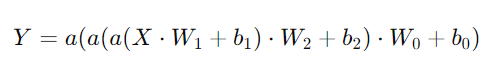
Y는 결국 함수의 계수이다.

딥 강화학습의 개념. State와 결과의 매칭이다.

데이터가 적으면 매핑이 안된다. Funtional Approximation이다.

함수의 관계를 만들기 위해서 결국 신경망을 만드는 것.

그래서 딥러닝은 데이터가 많을수록 성능이 안 좋을 수가 없다.

GAN Theory

There is a Pdata that represents the distribution of actual images

Pdata라고 하는 실제 이미지의 분포가 있다.

generative model의 목표는, 이 Pdata의 분포에 맞도록 Pmodel(x)의 값을 찾는 것이다.

따라서 Real 이미지를 훈련시켜, D(x)라는 결과는 1이 되도록 훈련시킨다.

이 녀석은 판별을 위한 Encoder 구조이다.(Discriminator)

순수한 이진분류기이다. 진짜인지 아닌지만 판단한다.

그리고 Fake는 random noise를 넣어 생성되는 Decoder의 형태를 띄고 있다.(Generator)

이 결과는 G(z)이다.

그렇게 Decoder에서 나온 값을 Encoder에 집어넣어서, 그 값의 오차가 적도록 하면,

한마디로 D(G(z))의 오차가 적도록 하면, Fake 이미지가 real 이미지와 같다는 뜻이 되고, 해당 분포(distribution)이 비슷하다는 듯이 된다.

이 log 1-D(G(z))는 cost 함수로서, 간단하게 cross entropy 함수와 같다고 생각하면 된다.

그러나 여기서의 cost 함수에는 이미 maximize, minimize가 정해져 있다.

log D(x)는 판별자의 에러이고, log(1-D(G(z)))는 생성자의 error이다.

-를 minimize 하느니, maximize 하는 게 더 쉬워서 이렇게 쓴다.

는 판별자가 실제 데이터를 올바르게 분류하는 확률을 최대화하는 데 기여하고,

l는 판별자가 생성된 데이터를 올바르게 분류하는 확률을 최대화하는 데 기여한다.

fake 판별 추정치는 최소화하고 싶고, max 판별 추정치는 최대화하고 싶다.

log D(G(z)) = Fake 판별 추정치

log (1-D(x)) = Real 판별 추정치

위의 확률을 최대화하고 싶다면, 반대로

생성자의 함수

arg minG Ez,x [log D(G(z)) + log (1-D(x)) ]

위의 확률을 최소화해서 loss 함수로 삼아주면 된다.

위 두개의 함수를 합친다.

arg minG maxD Ez,x [log D(G(z)) + log (1-D(x)) ]

그렇게 해서 나오는 함수이다.

PCA와 LDA

차원의 저주 : 차원이 너무 넓어지면 공간낭비와 시간낭비가 심하다.

그래서 적합 차원을 찾기 위해서는, 어떤 기준으로 잘라야 한다.

Feature Extraction은 어떠한 값에 대해서 어떤 행렬을 곱해서, 목적에 맞는 피처를 추출하는 것이다.

PCA = 아무리 차원을 축소해도 모양을 유지하는 것 > 투영

샘플의 특성을 유지하면서 차원을 축소시킨다.

LDA = 분류하기 쉬운 방향으로 차원을 축소하기 > 분류하기 쉽게 투영

모양이 유지되는지는 상관없다.

결정경계선이 유리하게 차원을 축소시킨다.

LDA는 그 자체로 클러스터링이 수행된다.

PCA 예시 : 얼굴의 특이점을 따서 각도를 추출한다.

LDA는 Maximize(평균1-평균2)^2 / (표준편차 제곱)

표준편차는 minimize하고, 평균의 차이는 Maximize해서 변환한다.

구현 관점에서는 VAE보다도, Dropout을 많이 쓴다.

내 블로그 - 관리자 홈 전환	`Q` `Q`
새 글 쓰기	`W` `W`

글 수정 (권한 있는 경우)	`E` `E`
댓글 영역으로 이동	`C` `C`

이 페이지의 URL 복사	`S` `S`
맨 위로 이동	`T` `T`
티스토리 홈 이동	`H` `H`
단축키 안내	`Shift` + `/` `⇧` + `/`

시카로의 공부방

티스토리 뷰