티스토리 뷰
주제
- 차량 공유업체의 차량 파손 여부 분류하기(이미지 데이터)
- 302개의 normal 데이터, 303개의 abnormal 데이터가 존재한다.
- 문제 정의
- 605개의 이미지 데이터가 있을 때, 파손 여부를 이진 분류할 수 있는 모델을 개발한다.
- 평가 함수 : Accuracy
목표
- 이미지 데이터 전처리 과정 실습
- 이미지 데이터 Augmentation 실습
- CNN, 전이학습 실습
- 모델 성능 향상을 위한 추가적인 하이퍼파라미터 설정, 다양한 전이학습 모델의 실습
프로젝트 내 역할
- 이미지 사이즈, learning_rate 및 weight_decay 반복 실험
- Sam(Sharpness-Aware Minimization) 시도
- sub-GAN 같은 Abnormal Detection에 대해서도 시도
- Cost가 적게 들어갈 것 같은 여러 전이 모델 실험
1. 데이터 분석
데이터 구성
- normal
- 1024*1024의 정상 차량 이미지 데이터
- abnormal
- 1024*1024의 파손된 차량 이미지 데이터
일단 1024*1024는 colab에서도 버티지 못하기 때문에, resize를 할 준비를 하고 들어간다.
2. 데이터 전처리
2.0 데이터 unzip하기
def dataset_extract(file_name) :
    with zipfile.ZipFile(file_name, 'r') as zip_ref :
        file_list = zip_ref.namelist()

        if os.path.exists(f'/content/{file_name[-14:-4]}/') :
            print(f'데이터셋 폴더가 이미 존재합니다.')
            return

        else :
            for f in tqdm(file_list, desc='Extracting', unit='files') :
                zip_ref.extract(member=f, path=f'./{file_name[-14:-4]}/')
2.1 개수 확인 및 y_label 만들기
개수를 확인하고, y_label을 만든다.
# 폴더별 이미지 데이터 갯수 확인
path = '/content/Car_Images/'

print( f'정상 차량 이미지 수 : {len(glob.glob(path+"normal/*"))}' )
print( f'파손 차량 이미지 수 : {len(glob.glob(path+"abnormal/*"))}' )

# 정상 차량은 0, 파손 차량은 1
y_normal = np.zeros((302,))
y_abnormal = np.ones((303,))

# 정상 차량 어레이와 파손 차량 어레이 합치기
y_total = np.hstack((y_normal, y_abnormal))
y_total.shape
2.2 데이터 Path 리스트를 통합하고, Train-Test 분리하기
glob을 사용하면 path를 통합할 수 있다.
이상탐지 및 이진분류 문제이고, 데이터가 얼마 없기 때문에, stratify를 주는 게 더 낫다고 판단하여 주었다.
x_total_list = glob.glob(path+"normal/*") + glob.glob(path+"abnormal/*")

from sklearn.model_selection import train_test_split

x_train,x_test,y_train,y_test = train_test_split(x_total_list,y_total,
                                                 test_size=0.2,
                                                 stratify=y_total,
                                                 random_state=2024)
x_test,x_val,y_test,y_val = train_test_split(x_test,
                                               y_test,
                                               test_size=0.5,
                                               stratify=y_test,
                                               random_state=2024)
2.3 Image to Array로 데이터를 array로 변환하기
여기가 핵심
다른 조들은 256, 128로 고정하면서 정확도를 늘렸는데, 나는 이미지 사이즈에 대한 학습 시간과 정확도가 궁금했다.
결론적으로 600*600일 때가 Colab이 버틸 수 있는 GPU의 한계였고, 이 상태에서 정확도를 늘려보기로 했다.
import keras
from keras.preprocessing import image
from keras.preprocessing.image import img_to_array #array 형태로 변환하는 방법
import numpy as np
from tqdm import tqdm

def x_preprocessing(img_list,width,height) :
    bin_list = []

    for img in tqdm(img_list) :
        img = keras.utils.load_img(img, color_mode='rgb',target_size=(width,height) )
        img = keras.utils.img_to_array(img)
        bin_list.append(img)

    return np.array(bin_list)

height=600
width=600

images = x_preprocessing(x_train,height,width)
images_test = x_preprocessing(x_test,height,width)
images_val = x_preprocessing(x_val,height,width)
2.4 전이학습을 위해 Scailing
각 전이학습 모델에서 제공하는 preprocess_input을 쓰면 괜찮다.
아니라면 직접 scailing 함수를 짜면 된다.
x_max, x_min = images.max(), images.min()
x_train_s = (images-x_min) / (x_max-x_min)
x_test_s = (images_test-x_min) / (x_max-x_min)
x_val_s = (images_val-x_min) / (x_max-x_min)

x_train_s.max(), x_train_s.min(), x_test_s.max(), x_test_s.min(),x_val_s.max(), x_val_s.min()

혹은

from keras.applications.inception_v3 import preprocess_input
from keras.applications.inception_v3 import InceptionV3

x_train_s = preprocess_input(images)
x_test_s = preprocess_input(images_test)
x_val_s = preprocess_input(images_val)

x_train_s.max(), x_train_s.min(), x_test_s.max(), x_test_s.min(),x_val_s.max(), x_val_s.min()
3. 딥러닝
3.0 전이학습 모델 설정
Efficienet, ResNet 등 여러 모델을 시도해보았으나, InceptionV3가 충분히 훈련시간 대비 정확도가 잘 나왔다.
그래서 해당 모델을 붙잡고 튜닝하는 게 낫다고 판단하여 진행했다.
trainable은 전부 false로 주었다. 원래 가중치를 활용하는 게 결과가 더 잘나왔다.
from keras.layers import Dense,Input,Flatten, Dropout, BatchNormalization,Conv2D,MaxPool2D,RandomFlip,RandomRotation,RandomTranslation,RandomZoom,RandomFlip
from keras.models import Model
from keras.callbacks import EarlyStopping
from keras.backend import clear_session

w,h,c = x_train_s.shape[1],x_train_s.shape[2],x_train_s.shape[3]

keras.backend.clear_session()

base_model = InceptionV3(weights='imagenet',       # ImageNet 데이터를 기반으로 미리 학습된 가중치 불러오기
                         include_top=False,

                         # InceptionV3 모델의 아웃풋 레이어는 제외하고 불러오기
                         input_shape= (w,h,c)) # 입력 데이터의 형태

base_model.trainable=False

for idx, layer in enumerate(base_model.layers):
    print(f"Layer {idx}: Trainable - {layer.trainable}")
3.1 전이학습 모델 설정2
기본적으로 쓰는 4개의 augmentation을 주었다.
0.1로 준 이유는 가장 보편적인 값이라서다.
Flip의 경우에는 일반화 성능을 높여줄 것 같아서 넣었다.
weight_decay를 줌으로서, L2 규제를 적용하여 훨씬 학습이 잘 되게 했다.
keras.backend.clear_session()

il = Input(shape=(w,h,c))
####################################
al = RandomRotation(factor=(-0.1,0.1))(il)
al = RandomTranslation(height_factor=(-0.1,0.1), width_factor=(-0.1,0.1))(al)
al = RandomZoom(height_factor=(-0.1,0.1), width_factor=(-0.1,0.1))(al)
al = RandomFlip(mode='horizontal_and_vertical')(al)


base_model = base_model(al)

new_output = GlobalAveragePooling2D()(base_model)
new_output = Dense(1, # class 3개   클래스 개수만큼 진행한다.
                  activation = 'sigmoid')(new_output)

model = keras.models.Model(il, new_output)
model.compile(optimizer=keras.optimizers.AdamW(weight_decay=0.01,learning_rate=0.0005),loss='binary_crossentropy',metrics=['accuracy'])

model.summary()
이 부분에서 논문에서 봤던 Sam(Sharpness-Aware Minimization) 을 활용해보기도 했다.
그러나 최대 성능이 1이 나와서 그런지 차이는 느끼지 못했다.
import tensorflow as tf
from tensorflow.keras.optimizers import Optimizer

class SAMOptimizer(Optimizer):
    def __init__(self, base_optimizer, rho=0.05, **kwargs):
        super(SAMOptimizer, self).__init__(learning_rate=0.0001,**kwargs)
        self.base_optimizer = base_optimizer
        self.rho = rho
        self.scope = None

    def set_scope(self, scope):
        self.scope = scope

    def get_updates(self, loss, params):
        base_optimizer = self.base_optimizer
        lr = base_optimizer.lr
        wd = base_optimizer.weight_decay

        grads = base_optimizer.get_gradients(loss, params)

        # Weight decay
        if wd != 0.:
            for p, g in zip(params, grads):
                g += wd * p

        # SAM update
        grads = [g * lr for g in grads]
        norm_grads = tf.linalg.global_norm(grads)

        scale = self.rho / (norm_grads + 1e-12)
        scaled_grads = [scale * g for g in grads]

        base_optimizer.apply_gradients(zip(scaled_grads, params))

        return self.base_optimizer.updates

    def get_config(self):
        config = {
            'base_optimizer': tf.keras.optimizers.serialize(self.base_optimizer),
            'rho': self.rho
        }
        base_config = super(SAMOptimizer, self).get_config()
        return dict(list(base_config.items()) + list(config.items()))
4. 결과
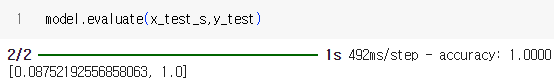
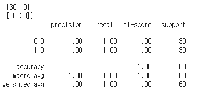
validset에 대해서 1이 나왔다.
다른 것 보다, 이미지 사이즈를 키운 게 컸다.
512*512에서도 0.96이었지만, 600으로 딱 맞추니 1이 떴다.
다만 train 시간은 확실히 이미지 사이즈를 작게 했을 때 보다 2~3배정도 오래 걸렸다. 용량도 256*256에 비해 2배 정도가 되는 걸 확인할 수 있었다.
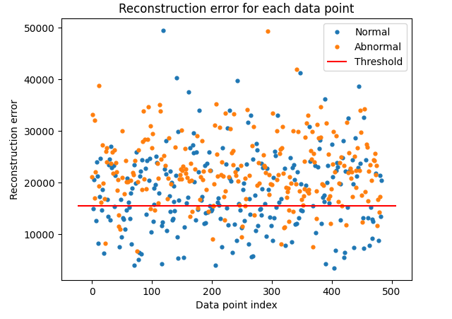
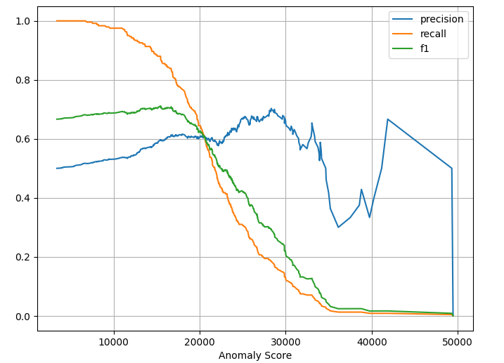
5. Anormaly Detection : Sub-GAN
이상탐지 문제이기 때문에, Sub-GAN을 활용한 Anormaly Detection도 수행해보았다.
from keras.layers import Dense,Input,Flatten, Dropout, BatchNormalization,Conv2D,MaxPool2D,RandomFlip,RandomRotation,RandomTranslation,RandomZoom,RandomFlip
from keras.models import Model
from keras.callbacks import EarlyStopping
from keras.backend import clear_session

clear_session()

# 하이퍼파라미터 설정
latent_dim = 128
input_size = (512, 512, 3)
batch_size = 4  # 배치 사이즈를 축소하여 GPU 메모리 부담을 줄입니다.
epochs = 50
lr = 0.0002

# Encoder 정의
encoder_input = Input(shape=input_size)

####################################
al = RandomRotation(factor=(-0.1,0.1))(encoder_input)
al = RandomTranslation(height_factor=(-0.1,0.1), width_factor=(-0.1,0.1))(al)
al = RandomZoom(height_factor=(-0.1,0.1), width_factor=(-0.1,0.1))(al)
al = RandomFlip(mode='horizontal_and_vertical')(al)

x = Conv2D(64, (4, 4), strides=(2, 2), padding='same')(al)
x = BatchNormalization()(x)
x = Activation('relu')(x)
x = Conv2D(128, (4, 4), strides=(2, 2), padding='same')(x)
x = BatchNormalization()(x)
x = Activation('relu')(x)
x = Conv2D(256, (4, 4), strides=(2, 2), padding='same')(x)
x = BatchNormalization()(x)
x = Activation('relu')(x)
x = Conv2D(512, (4, 4), strides=(2, 2), padding='same')(x)
x = BatchNormalization()(x)
x = Activation('relu')(x)
x = Flatten()(x)
encoder_output = Dense(latent_dim)(x)
encoder = Model(encoder_input, encoder_output)

# Decoder 정의
decoder_input = Input(shape=(latent_dim,))
x = Dense(32 * 32 * 512)(decoder_input)
x = Reshape((32, 32, 512))(x)
x = Conv2DTranspose(256, (4, 4), strides=(2, 2), padding='same')(x)
x = BatchNormalization()(x)
x = Activation('relu')(x)
x = Conv2DTranspose(128, (4, 4), strides=(2, 2), padding='same')(x)
x = BatchNormalization()(x)
x = Activation('relu')(x)
x = Conv2DTranspose(64, (4, 4), strides=(2, 2), padding='same')(x)
x = BatchNormalization()(x)
x = Activation('relu')(x)
x = Conv2DTranspose(3, (4, 4), strides=(2, 2), padding='same')(x)
decoder_output = Activation('sigmoid')(x)
decoder = Model(decoder_input, decoder_output)

# Sub-GAN 모델 정의
encoder_decoder = Model(encoder_input, decoder(encoder(encoder_input)))
optimizer = Adam(learning_rate=lr)
encoder_decoder.compile(optimizer=optimizer, loss='mse')

# 모델 학습
normal_vehicle_images =  x_normal_auto # 임시로 랜덤 데이터 생성
encoder_decoder.fit(normal_vehicle_images, normal_vehicle_images, batch_size=batch_size, epochs=epochs, shuffle=True, validation_split=0.2)
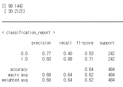
그러나 data augmentation까지 준 노력에 비해서, 결과가 굉장히 poor하게 나왔다.
강사님이 말하신 대로, 이미지 데이터의 편향성이 존재해서 그런 것 같다.
개인적인 인사이트
시각지능에서는 확실히 이미지 해상도가 가장 중요하다는 사실을 다시 한 번 상기했다.
그러나 On-Device에 적용하기 위해서는, 모델의 파라미터, 학습 시간, 메모리 사용량을 줄이는 기법(양자화 등)을 사용해서 정확도는 유지하면서 용량을 줄여야 할 것이다.
다른 조에게서 배운 점
keras에 있는 거의 모든 모델을 시도
RestNet50 ,EfficientNetB0가 좋은 accuracy 도출 - 0.96% 정도
Convnext 도 keras applications에서 제공
각 모델에 대해서 어떤 특징이 있는지 알아보고 그때 해당 모델들을 조금씩 같이 비교하면서 모델의 차이를 좀 보았으면 좋을 것 같다.
blur(흐림), Gaussian Blur, Sharpen(후추), Contrast Enhancement(선명도), Canny Edge Detection(배경을 없애고 객체들의 이미지에서 조금 더 객체 부각), Corner Detection(harris Corner)(모서리 부분 따오기)
cutmix 같은 강건성 늘리는 레이어도 알아두면 좋다.
각 레이어 하나당 논문 하나다.
이 조는 cv2에 있는 옵션들로 Data Augmentation을 활용했다.
Python
import cv2
import numpy as np
from tqdm import tqdm

def apply_augmentations(img_array):
    augmentations = []

    # Blur
    blur = cv2.blur(img_array, (5, 5))
    augmentations.append(blur)

    # Gaussian Blur
    gaussian_blur = cv2.GaussianBlur(img_array, (5, 5), 0)
    augmentations.append(gaussian_blur)

    # Sharpen
    kernel_sharpen = np.array([[-1, -1, -1, -1, 9, -1, -1, -1, -1]])
    sharpen = cv2.filter2D(img_array, -1, kernel_sharpen)
    augmentations.append(sharpen)

    # Contrast Enhancement
    contrast = exposure.equalize_adapthist(img_array/255.0)
    contrast = np.clip(contrast * 255.0, 0, 255).astype('uint8')
    augmentations.append(contrast)

    # Canny Edge Detection
    edges = cv2.Canny(img_array.astype(np.uint8), 100, 200)
    augmentations.append(edges)

    # Corner Detection (Harris Corner)
    gray = cv2.cvtColor(img_array.astype(np.uint8), cv2.COLOR_RGB2GRAY)
    corners = cv2.cornerHarris(gray, 2, 3, 0.04)
    corners = cv2.dilate(corners, None)
    corners = np.stack((corners,) * 3, axis=-1)
    augmentations.append(corners)

    return augmentations

def augment_dataset(dataset):
    augmented_data = []

    for img_array, label in tqdm(dataset, total=len(dataset)):
        augmentations = apply_augmentations(img_array)

        for aug_img in augmentations:
            augmented_data.append((aug_img, label))

    return np.array(augmented_data, dtype=object)

# ...

augmented_train_dataset = augment_dataset(train_dataset)
https://keras.io/api/keras_cv/layers/
keras CV라는 layer가 다 따로 있다.
2번쪠 조
CNN - 82%
ResNet50 - 77%
EfficientNetB4 - 90%
InceptionV3 - 98.96%(내가 한 결론과 같다)
resnet block을 구현
import tensorflow as tf

def resnet_block(input_tensor, filters, strides=(1, 1)):
    """
    ResNet 블록 정의

    Args:
        input_tensor: 입력 텐서
        filters: 필터 수
        strides: 스트라이드

    Returns:
        ResNet 블록의 출력 텐서
    """

    x = tf.keras.layers.Conv2D(filters, (3, 3), strides=strides, padding='same')(input_tensor)
    x = tf.keras.layers.BatchNormalization()(x)
    x = tf.keras.layers.Activation('relu')(x)

    x = tf.keras.layers.Conv2D(filters, (3, 3), padding='same')(x)
    x = tf.keras.layers.BatchNormalization()(x)

    if strides != (1, 1):
        shortcut = tf.keras.layers.Conv2D(filters, (1, 1), strides=strides)(input_tensor)
        shortcut = tf.keras.layers.BatchNormalization()(shortcut)
    else:
        shortcut = input_tensor

    x = tf.keras.layers.Add()([x, shortcut])
    x = tf.keras.layers.Activation('relu')(x)

    return x

def resnet50(input_shape, num_classes=1):
    """
    ResNet50 모델 구성

    Args:
        input_shape: 입력 데이터 형식
        num_classes: 분류할 클래스 수

    Returns:
        ResNet50 모델
    """

    inputs = tf.keras.Input(shape=input_shape)

    x = tf.keras.layers.Conv2D(64, (7, 7), strides=(2, 2), padding='same')(inputs)
    x = tf.keras.layers.BatchNormalization()(x)
    x = tf.keras.layers.Activation('relu')(x)
    x = tf.keras.layers.MaxPooling2D((3, 3), strides=(2, 2), padding='same')(x)

    # 4개의 ResNet 블록 그룹
    for filters, num_blocks in zip([64, 128, 256, 512], [3, 4, 6, 3]):
        for i in range(num_blocks):
            x = resnet_block(x, filters)

    x = tf.keras.layers.GlobalAveragePooling2D()(x)
    x = tf.keras.layers.Dense(num_classes, activation='softmax')(x)

    model = tf.keras.Model(inputs=inputs, outputs=x)

    return model

# ...

model = resnet50((224, 224, 3))
model.compile(optimizer='adam',
              loss='sparse_categorical_crossentropy',
              metrics=['accuracy'])

model.fit(train_data, train_labels, epochs=10)

model.evaluate(test_data, test_labels)
모델 구조를 보고서 직접 따라 만들 수 있어야 한다.
3번째 조
imagedata augmentation - imagedata generator를 썼다.
언젠가 사라질 것을 알고 있기에 강사님은 안 썼다.
keras의 지향 방향 - 모델 구조 내에서 모든 걸 해결하고 싶어 한다.
여러 개 모델을 전부 fit해서 DenseNet으로 시간, 정확도를 전부 구해서 나열했다.
DeepSVDD - one class classification / Anomaly Detection 구현
pytorch로 되어 있다 보니까 구현하기 힘들어서 불가능
강사님의 추가 강의
Activation = 'swish' => google에서 주장하고 있는 activation. relu보다 성능이 좋다고 얘기한다.
from keras.utils import image_dataset_from_directory

idfd_Train, idfd_valid =image_dataset_from_directory('path',
	label_mode='binary',
    image_size=(128,128),
    shuffle=True,
    seed=2024,
    validation_split=0.2,
    subset='both' )
base_model.trainable=False
모델 성능
https://keras.io/api/applications/
Keras에서 사용가능한 총 파라미터가 몇개인지 전부 나와 있다.
4차 미니프로젝트 1,2일차를 마치며
벌써 4차가 되었고, 수업을 들은지도 2달이 지났다.
개인적으로 미니프로젝트를 준비하면서 보았던 논문들이 굉장히 재미있었다. Sam, Venom, EfficeinetL2 등등..
컴퓨터 비전 분야가 2년 안에 정복된다는 말도 있지만, 내가 보기엔 아직 멀어보인다. 현대 컴퓨터 비전 연구는 사실 이미지의 해상도가 적은 상태에서도 쓸 수 있는 모델이 백미이다. 메모리가 적게 들고, 무엇보다 빠르니까.
Classification에서는 그럴듯한 정확도를 자랑하지만, Data Auggmentation이나 Object Detection 같은 세부 분야에서는 논문거리도 많다.
그렇기에 이런 기법들을 로봇에까지 적용할 수 있도록 나는 공부를 더 멈추지 않을 생각이다. 무엇보다 재미있으니까.